what is consider large mean for poisson random variable to be consider normal distributed
The Poisson Distribution and Poisson Process Explained
A straightforward walk-through of a useful statistical concept
A tragedy of statistics in most schools is how dull information technology's made. Teachers spend hours wading through derivations, equations, and theorems, and, when yous finally get to the best part — applying concepts to actual numbers — it'due south with irrelevant, unimaginative examples like rolling dice. This is a shame every bit stats tin can be enjoyable if you skip the derivations (which yous'll likely never need) and focus on using the ideas to solve interesting problems.
In this article, we'll cover Poisson Processes and the Poisson distribution, two important probability concepts. After highlighting merely the relevant theory, nosotros'll work through a real-earth example, showing equations and graphs to put the ideas in a proper context.
Poisson Process
A Poisson Process is a model for a series of detached event where the average fourth dimension between events is known, but the exact timing of events is random. The inflow of an event is independent of the upshot before (waiting time betwixt events is memoryless). For example, suppose we ain a website which our content delivery network (CDN) tells united states of america goes down on boilerplate in one case per 60 days, only one failure doesn't affect the probability of the next. All nosotros know is the average fourth dimension between failures. This is a Poisson process that looks like:
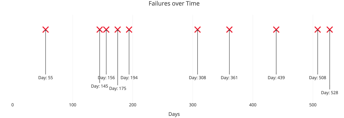
The important point is nosotros know the average time between events but they are randomly spaced (stochastic). Nosotros might have back-to-back failures, simply nosotros could also go years between failures due to the randomness of the process.
A Poisson Process meets the following criteria (in reality many phenomena modeled as Poisson processes don't encounter these exactly):
- Events are independent of each other. The occurrence of i event does non touch the probability another upshot volition occur.
- The average rate (events per time period) is constant.
- 2 events cannot occur at the aforementioned time.
The final point — events are not simultaneous — ways nosotros can think of each sub-interval of a Poisson process as a Bernoulli Trial, that is, either a success or a failure. With our website, the unabridged interval may be 600 days, but each sub-interval — 1 day — our website either goes down or it doesn't.
Mutual examples of Poisson processes are customers calling a help middle, visitors to a website, radioactivity in atoms, photons arriving at a infinite telescope, and movements in a stock price. Poisson processes are mostly associated with time, just they exercise not have to exist. In the stock instance, we might know the boilerplate movements per day (events per fourth dimension), just we could also have a Poisson process for the number of trees in an acre (events per area).
(One instance frequently given for a Poisson Process is motorbus arrivals (or trains or at present Ubers). Yet, this is not a true Poisson procedure because the arrivals are not independent of ane some other. Even for bus systems that do not run on time, whether or not one motorbus is tardily affects the arrival time of the side by side bus. Jake VanderPlas has a great article on applying a Poisson process to bus arrival times which works better with made-up information than real-world data.)
Poisson Distribution
The Poisson Process is the model we use for describing randomly occurring events and by itself, isn't that useful. We need the Poisson Distribution to exercise interesting things like finding the probability of a number of events in a time period or finding the probability of waiting some fourth dimension until the next result.
The Poisson Distribution probability mass function gives the probability of observing chiliad events in a time menstruum given the length of the period and the average events per time:

This is a fiddling convoluted, and events/time * fourth dimension flow is usually simplified into a single parameter, λ, lambda, the rate parameter. With this substitution, the Poisson Distribution probability part now has one parameter:

Lambda tin exist thought of equally the expected number of events in the interval. (Nosotros'll switch to calling this an interval because remember, nosotros don't accept to use a time menses, nosotros could use surface area or book based on our Poisson process). I similar to write out lambda to remind myself the rate parameter is a function of both the boilerplate events per time and the length of the time menstruum simply yous'll most commonly see it as direct higher up.
As nosotros modify the rate parameter, λ, nosotros change the probability of seeing different numbers of events in 1 interval. The below graph is the probability mass role of the Poisson distribution showing the probability of a number of events occurring in an interval with unlike rate parameters.
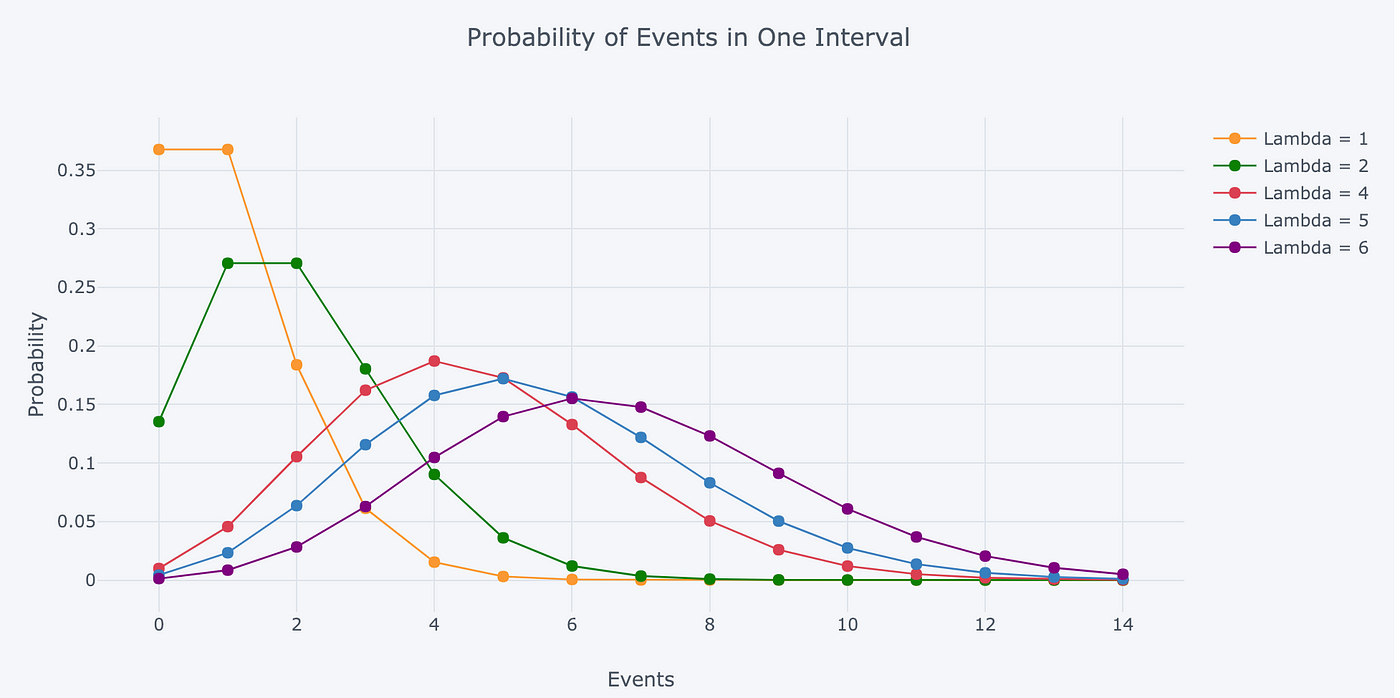
The most likely number of events in the interval for each curve is the rate parameter. This makes sense because the rate parameter is the expected number of events in the interval and therefore when it'due south an integer, the rate parameter will be the number of events with the greatest probability.
When it's not an integer, the highest probability number of events will be the nearest integer to the rate parameter, since the Poisson distribution is but divers for a discrete number of events. The discrete nature of the Poisson distribution is also why this is a probability mass function and non a density function. (The rate parameter is also the hateful and variance of the distribution, which practice not demand to be integers.)
We tin use the Poisson Distribution mass role to notice the probability of observing a number of events over an interval generated past a Poisson process. Another use of the mass role equation — every bit nosotros'll see later — is to detect the probability of waiting some time betwixt events.
A Worked-Out Instance
For the problem we'll solve with a Poisson distribution, nosotros could continue with website failures, but I propose something grander. In my babyhood, my father would oftentimes take me into our yard to observe (or try to observe) meteor showers. We were not space geeks, but watching objects from outer space burn up in the sky was enough to get u.s.a. outside even though meteor showers always seemed to occur in the coldest months.
The number of meteors seen tin can be modeled as a Poisson distribution because the meteors are contained, the boilerplate number of meteors per hour is constant (in the short term), and — this is an approximation — meteors don't occur simultaneously. To narrate the Poisson distribution, all we demand is the rate parameter which is the number of events/interval * interval length. From what I call up, we were told to expect 5 meteors per 60 minutes on average or 1 every 12 minutes. Due to the limited patience of a young kid (especially on a freezing nighttime), we never stayed out more than hr, and then nosotros'll employ that equally the fourth dimension period. Putting the 2 together, we get:

What exactly does "5 meteors expected" mean? Well, according to my pessimistic dad, that meant nosotros'd run across three meteors in an hour, tops. At the fourth dimension, I had no information science skills and trusted his judgment. Now that I'm older and have a healthy amount of skepticism towards authorization figures, it's time to put his statement to the examination. Nosotros can employ the Poisson distribution to find the probability of seeing exactly 3 meteors in i hour of ascertainment:

14% or about i/7. If nosotros went outside every night for 1 week, then nosotros could expect my dad to be correct precisely one time! While that is nice to know, what we are after is the distribution, the probability of seeing dissimilar numbers of meteors. Doing this past hand is tedious, so we'll use Python — which you lot tin run into in this Jupyter Notebook — for calculation and visualization.
The below graph shows the Probability Mass Office for the number of meteors in an hour with an average time between meteors of 12 minutes (which is the aforementioned every bit saying 5 meteors expected in an hour).
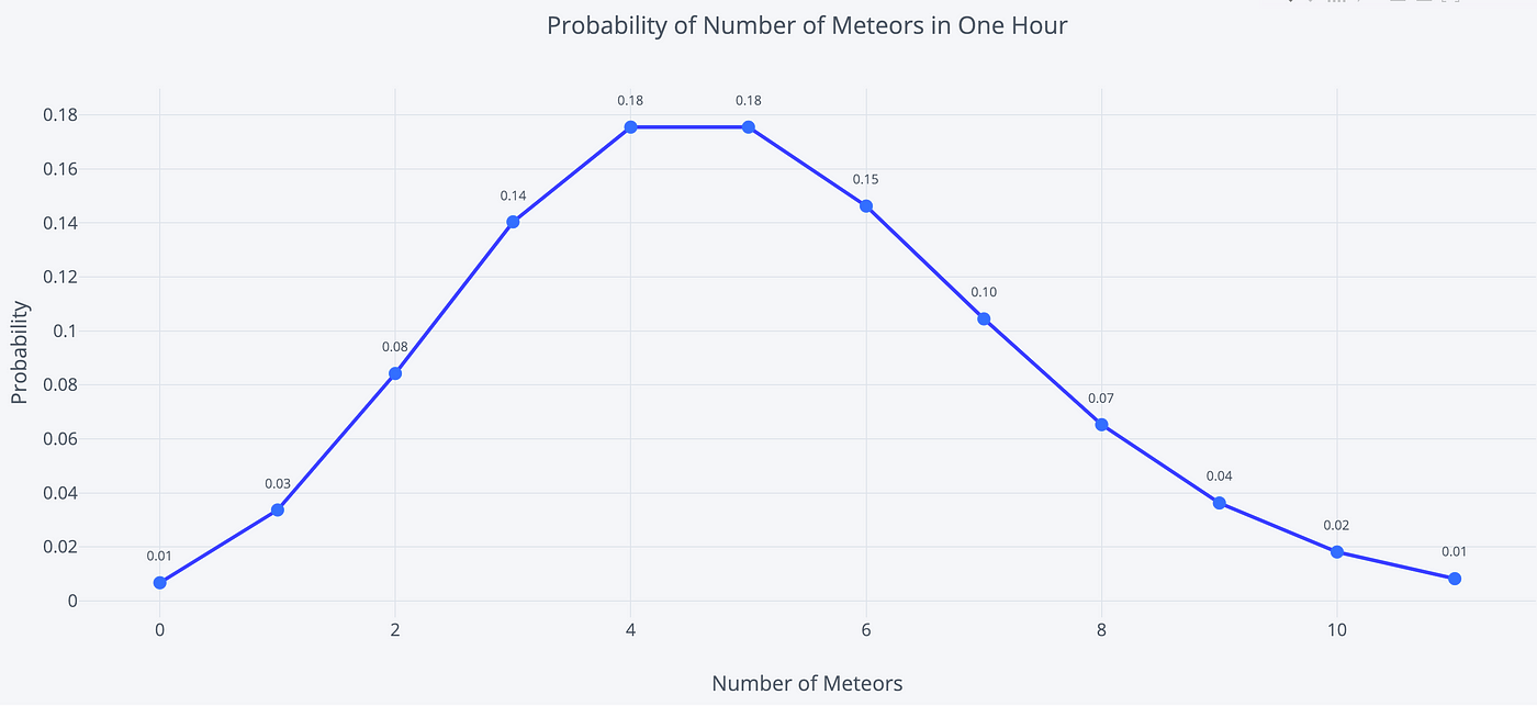
This is what "5 expected events" ways! The most likely number of meteors is 5, the rate parameter of the distribution. (Due to a quirk of the numbers, four and 5 have the same probability, eighteen%). As with any distribution, at that place is one virtually likely value, but there are also a wide range of possible values. For instance, we could go out and meet 0 meteors, or we could meet more ten in one 60 minutes. To find the probabilities of these events, we use the same equation but this time summate sums of probabilities (see notebook for details).
We already calculated the chance of seeing exactly iii meteors as about xiv%. The take a chance of seeing 3 or fewer meteors in 1 hr is 27% which means the probability of seeing more than three is 73%. Besides, the probability of more than than 5 meteors is 38.iv% while we could wait to meet five or fewer meteors in 61.half dozen% of observation hours. Although it's small, there is a ane.iv% hazard of observing more than 10 meteors in an 60 minutes!
To visualize these possible scenarios, we tin run an experiment by having our sister record the number of meteors she sees every hour for ten,000 hours. The results are shown in the histogram below:
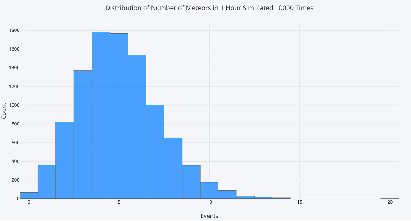
(This is obviously a simulation. No sisters were employed for this article.) Looking at the possible outcomes reinforces that this is a distribution and the expected outcome does non ever occur. On a few lucky nights, we'd witness ten or more meteors in an hour, although we'd usually come across 4 or 5 meteors.
Experimenting with the Rate Parameter
The rate parameter, λ, is the only number we need to ascertain the Poisson distribution. Yet, since it is a product of two parts (events/interval * interval length) there are two ways to alter it: nosotros can increment or decrease the events/interval and we can increment or subtract the interval length.
First, let's change the charge per unit parameter by increasing or decreasing the number of meteors per hour to see how the distribution is affected. For this graph, we are keeping the time period constant at 60 minutes (1 hour).
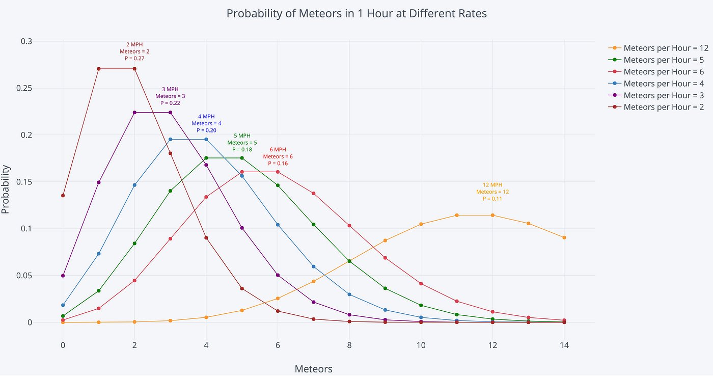
In each instance, the most likely number of meteors over the 60 minutes is the expected number of meteors, the rate parameter for the Poisson distribution. Equally one example, at 12 meteors per 60 minutes (MPH), our rate parameter is 12 and at that place is an xi% chance of observing exactly 12 meteors in 1 hour. If our rate parameter increases, we should wait to see more meteors per hr.
Some other pick is to increase or decrease the interval length. Below is the same plot, but this time we are keeping the number of meteors per hour constant at five and changing the length of time we observe.
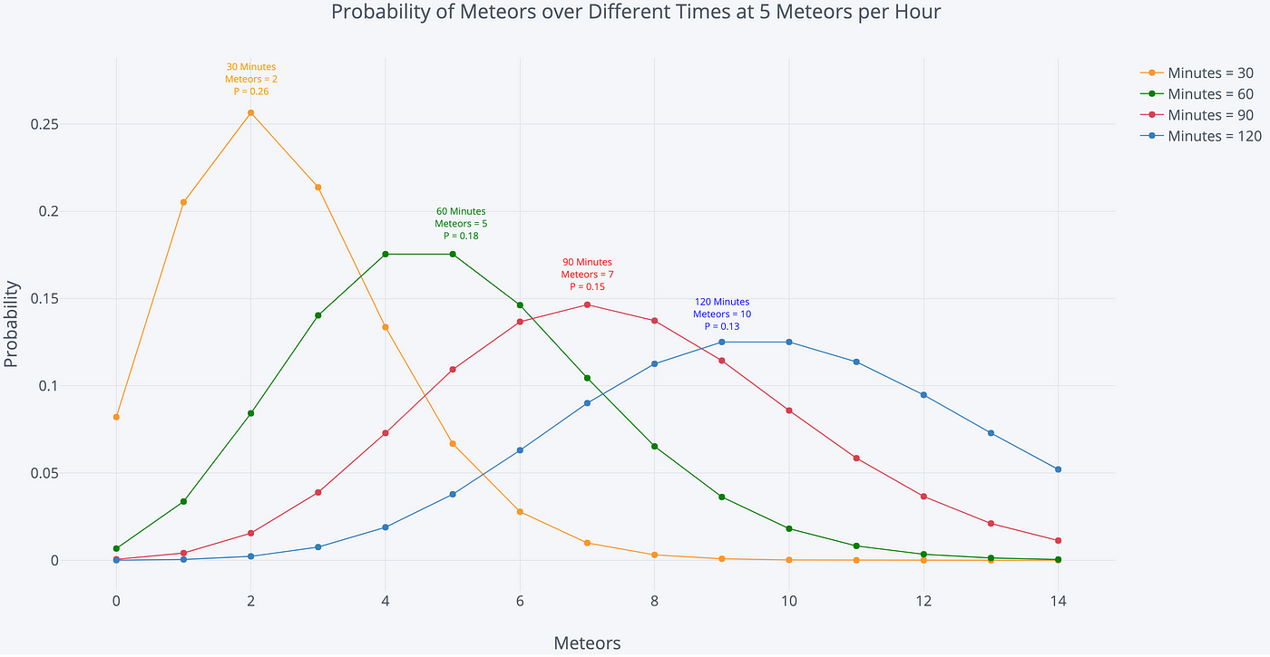
Information technology's no surprise that we await to meet more meteors the longer nosotros stay out! Whoever said "he who hesitates is lost" conspicuously never stood around watching falling star showers.
Waiting Time
An intriguing part of a Poisson process involves figuring out how long we have to wait until the adjacent event (this is sometimes called the interarrival fourth dimension). Consider the state of affairs: meteors appear once every 12 minutes on average. If nosotros arrive at a random time, how long can we look to wait to come across the next meteor? My dad always (this fourth dimension optimistically) claimed we but had to wait half-dozen minutes for the first meteor which agrees with our intuition. Still, if we've learned anything, information technology's that our intuition is not proficient at probability.
I won't go into the derivation (it comes from the probability mass function equation), but the time we can await to wait between events is a decomposable exponential. The probability of waiting a given amount of time between successive events decreases exponentially as the fourth dimension increases. The following equation shows the probability of waiting more than than a specified time.

With our example, we have ane event/12 minutes, and if we plug in the numbers we get a 60.65% chance of waiting > 6 minutes. Then much for my dad's judge! To prove some other case, we can wait to wait more than 30 minutes about 8.2% of the time. (We demand to note this is between each successive pair of events. The waiting times betwixt events are memoryless, so the fourth dimension between two events has no outcome on the fourth dimension between any other events. This memorylessness is too known as the Markov belongings).
A graph helps the states to visualize the exponential decay of waiting fourth dimension:
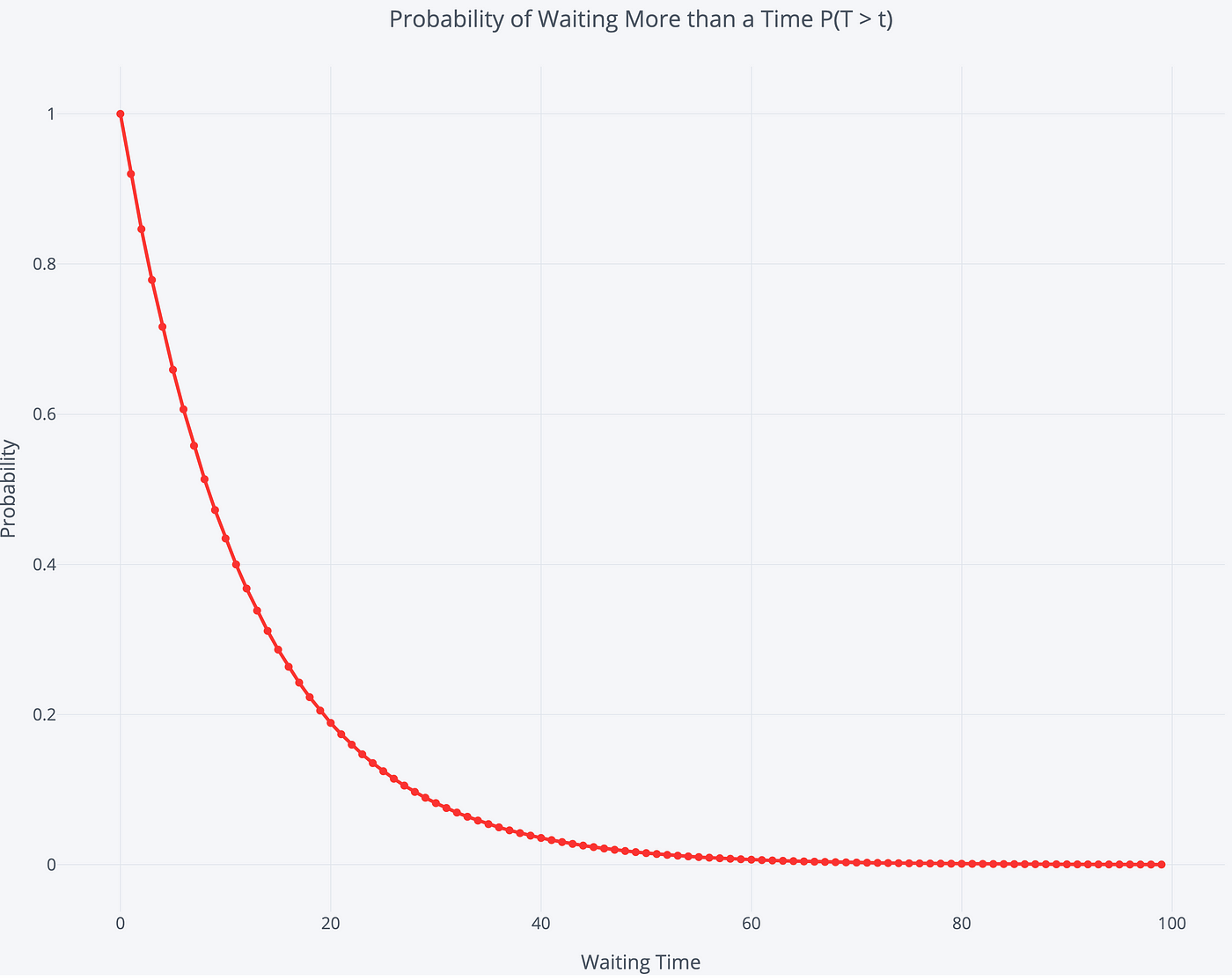
In that location is a 100% hazard of waiting more than 0 minutes, which drops off to a virtually 0% chance of waiting more than than 80 minutes. Again, since this is a distribution, there are a wide range of possible interarrival times.
Conversely, we tin utilise this equation to find the probability of waiting less than or equal to a time:

We can expect to await 6 minutes or less to meet a meteor 39.4% of the fourth dimension. We tin also find the probability of waiting a menses of time: in that location is a 57.72% probability of waiting between 5 and 30 minutes to see the next meteor.
To visualize the distribution of waiting times, nosotros can once more run a (simulated) experiment. We simulate watching for 100,000 minutes with an average rate of 1 falling star / 12 minutes. And then, we detect the waiting time betwixt each falling star nosotros see and plot the distribution.
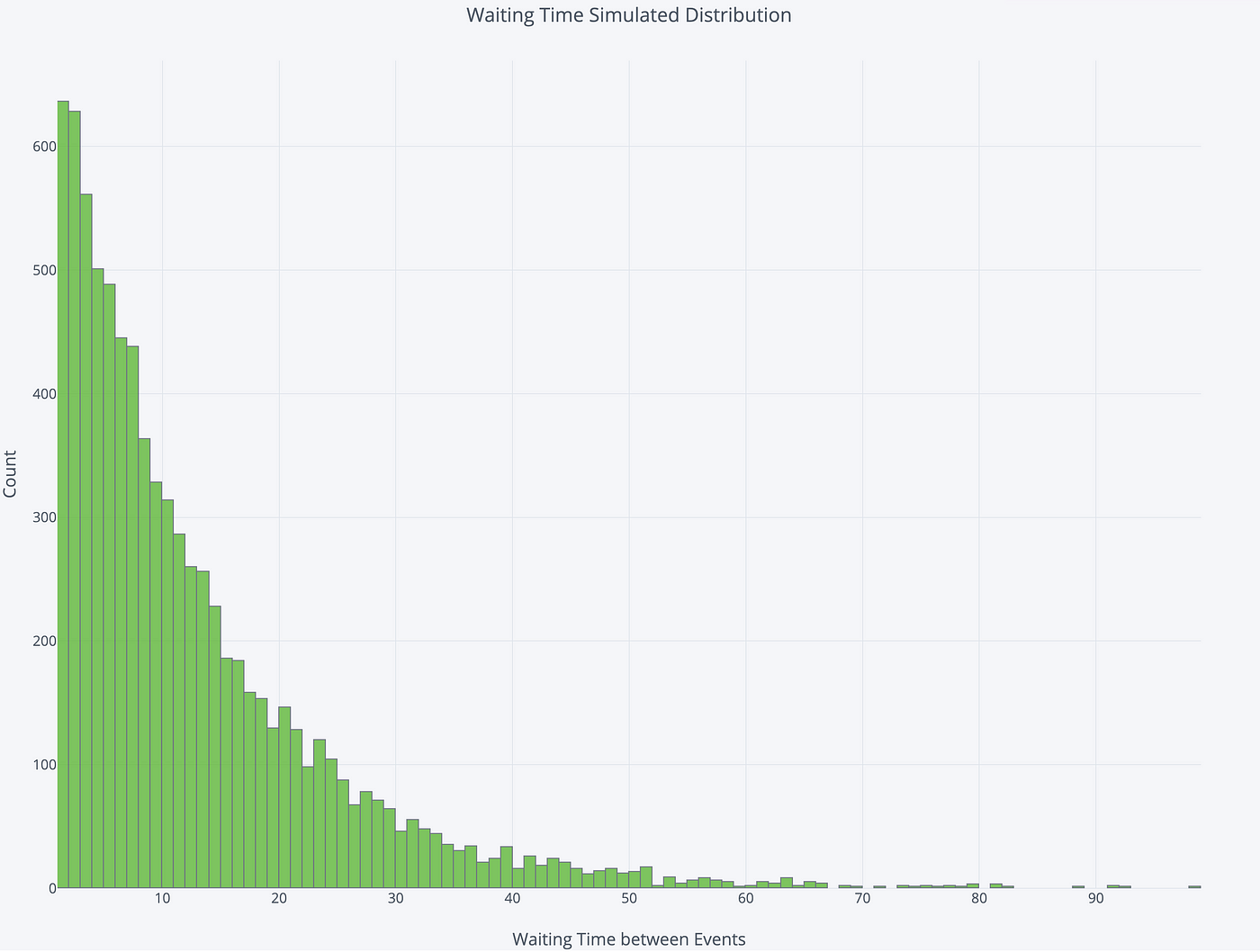
The virtually likely waiting fourth dimension is 1 infinitesimal, but that is non the average waiting fourth dimension. Let's get back to the original question: how long can nosotros wait to wait on average to encounter the first meteor if we make it at a random time?
To respond the average waiting fourth dimension question, we'll run 10,000 separate trials, each time watching the sky for 100,000 minutes. The graph beneath shows the distribution of the average waiting time between meteors from these trials:
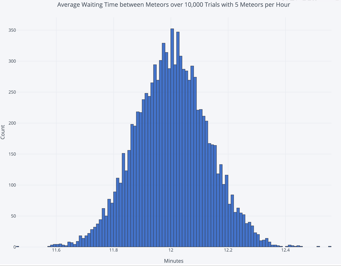
The average of the 10,000 averages turns out to be 12.003 minutes. Even if we get in at a random time, the average time we tin await to wait for the first shooting star is the average time between occurrences. At first, this may exist hard to understand: if events occur on average every 12 minutes, then why should we accept to wait the entire 12 minutes before seeing one event? The reply is this is an average waiting time, taking into business relationship all possible situations.
If the meteors came exactly every 12 minutes, then the average time we'd have to wait to see the beginning one would exist 6 minutes. However, because this is an exponential distribution, sometimes we show up and have to wait an hour, which outweighs the greater number of times when we wait fewer than 12 minutes. This is called the Waiting Time Paradox and is a worthwhile read.
As a final visualization, permit'southward do a random simulation of ane hour of observation.
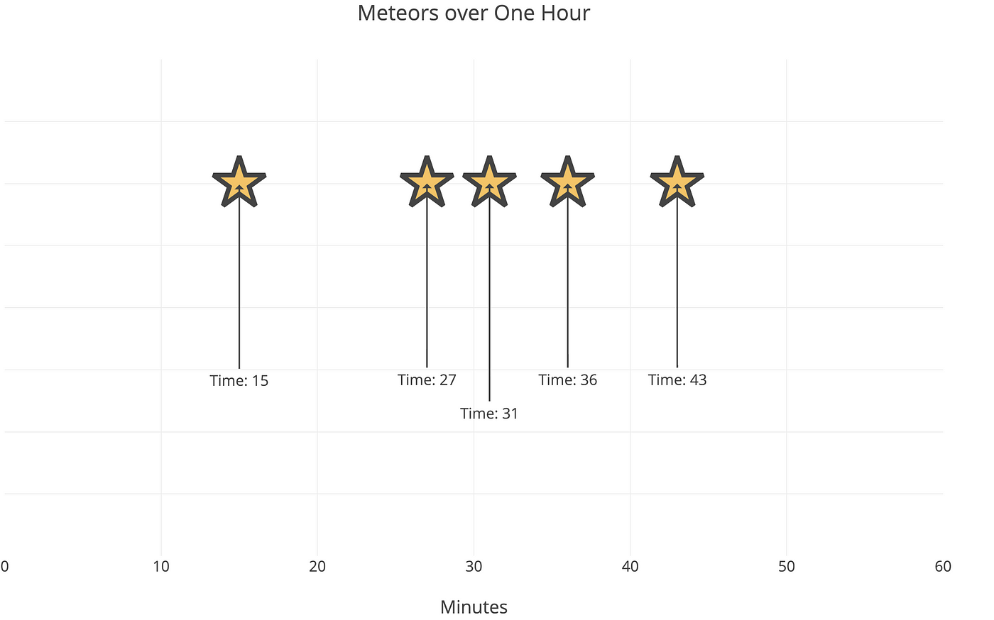
Well, this time nosotros got exactly what we expected: 5 meteors. We had to wait xv minutes for the outset one, just and then had a proficient stretch of shooting stars. At least in this case, it'd exist worth going out of the firm for celestial observation!
Notes on Poisson Distribution and Binomial Distribution
A Binomial Distribution is used to model the probability of the number of successes nosotros tin expect from n trials with a probability p. The Poisson Distribution is a special case of the Binomial Distribution every bit n goes to infinity while the expected number of successes remains fixed. The Poisson is used equally an approximation of the Binomial if n is large and p is small.
Every bit with many ideas in statistics, "big" and "minor" are up to interpretation. A rule of thumb is the Poisson distribution is a decent approximation of the Binomial if due north > 20 and np < 10. Therefore, a coin flip, even for 100 trials, should be modeled equally a Binomial because np =50. A telephone call centre which gets 1 telephone call every 30 minutes over 120 minutes could be modeled as a Poisson distribution equally np = 4. 1 important distinction is a Binomial occurs for a fixed set of trials (the domain is discrete) while a Poisson occurs over a theoretically infinite number of trials (continuous domain). This is only an approximation; recall, all models are wrong, merely some are useful!
For more than on this topic, see the Related Distribution section on Wikipedia for the Poisson Distribution. There is likewise a practiced Stack Exchange answer here.
Notes on Meteors/Meteorites/Meteoroids/Asteroids
Meteors are the streaks of light you lot meet in the sky that are acquired past pieces of debris called meteoroids burning upwardly in the atmosphere. A meteoroid tin come from an asteroid, a comet, or a piece of a planet and is usually millimeters in diameter simply can be upward to a kilometer. If the meteoroid survives its trip through the atmosphere and impacts Earth, information technology's chosen a meteorite. Asteroids are much larger chunks of rock orbiting the sun in the asteroid belt. Pieces of asteroids that pause off become meteoroids. The more yous know!.
Conclusions
To summarize, a Poisson Distribution gives the probability of a number of events in an interval generated by a Poisson process. The Poisson distribution is defined by the rate parameter, λ, which is the expected number of events in the interval (events/interval * interval length) and the highest probability number of events. We tin also apply the Poisson Distribution to find the waiting time between events. Even if we arrive at a random fourth dimension, the average waiting time will always exist the boilerplate time between events.
The side by side time you find yourself losing focus in statistics, you have my permission to stop paying attending to the teacher. Instead, find the relevant equations and apply them to an interesting trouble. You can learn the textile and yous'll have an appreciation for how stats helps us to empathise the world. Above all, stay curious: there are many amazing phenomenon in the world, and we can use data science is a bully tool for exploring them,
Equally always, I welcome feedback and constructive criticism. I can exist reached on Twitter @koehrsen_will.
Source: https://towardsdatascience.com/the-poisson-distribution-and-poisson-process-explained-4e2cb17d459
0 Response to "what is consider large mean for poisson random variable to be consider normal distributed"
Post a Comment